Project 4: CS61kaChow

Deadline: Tuesday, April 23, 11:59:59 PM PT

For this project, remember that the verb form of convolution is "convolve" not "convolute". Convolute means to complicate things, but in case you forget, here's a helpful quote:

"Convolute is what I do on exams, convolve is what you do on exams."

-Babak Ayazifar, EE120 Professor

Introduction

One of the major goals of this project is to explore how to speed up our programs. However, as with any real-world performance tests, there are many different factors that can affect the performance of any particular program.

For this project, one of the greatest factors is the load on the hive machines. Heavy hive machine load may significantly affect execution time and speedup. In fact, it can drastically misrepresent the performance of your program, when in fact your code may be correct.

As a result, we recommend the following in order to get the most consistent results from running your tests on the hive:

1. Start working on the project early. Inevitably, more students will be working on the project closer to the deadline. As such, students who start early will have a higher chance of using the hive machines under lower amounts of load.
2. Check Hivemind to choose which hive machine to ssh into. You will want to select a hive machine that has a low overall load, CPU usage, and number of current users.
3. Try working on the project during times that other students are not working. You will find that certain hours of the day have less average hive machine load; running your tests during this time will help you get more consistent performance results.

Setup: Git

This assignment can be done alone or with a partner.

If there are extenuating circumstances that require a partner switch (e.g. your partner drops the class, your partner is unresponsive), please reach out to us privately.

1. Visit Gradar. Log in and register your Project 4 group (and add your partner, if you have one), then create a GitHub repo for you or your group. If you have a partner, one partner should create a group and invite the other partner to that repo. The other partner should accept the invite without creating their own group.

2. Clone the repository on a hive machine.

   git clone git@github.com:61c-student/sp24-proj4-USERNAME.git 61c-proj4
   

   (replace username with your GitHub username)

3. Navigate to your repository:

   cd 61c-proj4
   

4. Add the starter repository as a remote:

   git remote add starter https://github.com/61c-teach/sp24-proj4-starter.git
   

If you run into git issues, please check out the common errors page.

Setup: Testing

The starter code does not come with any provided tests. To download the staff tests, run the following command:

python3 tools/create_tests.py

Background

This section is a bit long, so feel free to skip it for now, but please refer to them as needed since they provide helpful background information for the tasks in this project.

Convolutions

For background information about what a convolution is and why it is useful, see Appendix: (Optional) Convolutions.

Application: Video Processing

For this project, we will be applying convolutions to a real world application: video processing. Convolutions can blur, sharpen, or apply other effects to videos. This is possible because individual frames in a video can be treated as matrices of red, blue, and green values constructing the color for a given pixel. For simplicity, we're only working with grayscale videos, so that there's only one value per pixel (as opposed to one value for red, one for green, one for blue). As such, we can perform any matrix operation on each video frame, one of them being convolution.

When we convolve a matrix with an image, the matrix we use will have a major impact on the outcome ranging from sharpening to blurring an image. The matrices that we provide in this project will blur or sharpen your video frames. For each pixel, we compute a weighted average using the pixel itself and the pixels near it. By averaging many pixels together, this will smoothen any difference between their values, resulting in a blur. This is referred to as “Gaussian Blur” and is exactly how your phone blurs photos.

Vectors

In this project, a vector is represented as an array of int32_ts, or a int32_t *.

Matrices

In this project, we provide a type matrix_t defined as follows:

typedef struct {
  uint32_t rows;
  uint32_t cols;
  int32_t *data;
} matrix_t;

In matrix_t, rows represents the number of rows in the matrix, cols represents the number of columns in the matrix, and data is a 1D array of the matrix stored in row-major format (similar to project 2). For example, the matrix [[1, 2, 3], [4, 5, 6]] would be stored as [1, 2, 3, 4, 5, 6].

bin files

Matrices are stored in .bin files as a consecutive sequence of 4-byte integers (identical to project 2). The first and second integers in the file indicate the number of rows and columns in the matrix, respectively. The rest of the integers store the elements in the matrix in row-major order.

To view matrix files, you can run xxd -e matrix_file.bin, replacing matrix_file.bin with the matrix file you want to read. The output should look something like this:

00000000: 00000003 00000003 00000001 00000002  ................
00000010: 00000003 00000004 00000005 00000006  ................
00000020: 00000007 00000008 00000009           ............

The left-most column indexes the bytes in the file (e.g. the third row starts at the 0x20th byte of the file). The dots on the right display the bytes in the file as ASCII, but these bytes don't correspond to printable ASCII characters so only dot placeholders appear.

The actual contents of the file are listed in 4-byte blocks, with 4 blocks displayed per row. The first row has the numbers 3 (row count), 3 (column count), 1 (first element), and 2 (second element). This is a 3x3 matrix with elements [1, 2, 3, 4, 5, 6, 7, 8, 9].

Task

In this project, we provide a type task_t defined as follows:

typedef struct {
  char *path;
} task_t;

Each task represents a convolution operation (we'll go into what convolution is later), and is uniquely identified by its path. The path member of the task_t struct is the relative path to the folder containing the task.

Testing Framework

Tests in this project are located in the tests directory. The starter code does not contain any tests, but it contains a script tools/create_tests.py which will create the tests directory and generate tests. If you would like to make a custom test, please add it to tools/custom_tests.py. Feel free to use the tests we provide in tools/staff_tests.py as examples.

Once you define a custom test in custom_tests.py, you can run the test using the make commands provided in the task that you're currently working on, and the test will be generated for you based on the parameters you specify.

Directory Structure

Here's what folder should look like after running the example above:

61c-proj4/ # Your root project 4 folder
├─src/     # Where your source files are located
├─tests/   # Where your test files are located
│ └─my_custom_test/ # Where a specific test is located
│   ├─input.txt    # The input file to pass to your program, contains the number of tasks and task path
│   ├─task0/        # The first task
│   │ ├─a.bin         # Matrix A used in this task
│   │ ├─b.bin         # Matrix B used in this task
│   │ ├─ref.bin       # Reference output matrix generated by our script
│   │ └─out.bin       # Output matrix generated by your program
│   ├─task1/        # The second task, with the same folder structure
│   ├─...
│   └─task9/        # The tenth (last) task
├─tools/   # Where some utility scripts are stored
└─Makefile # Makefile for compilation and running the program.

The path member of the task_t struct for task0 would be would be tests/my_custom_test/task0.

Testing

This project uses a Makefile for running tests. The Makefile accepts one variable: TEST. TEST should be a path to a folder in tests/ that contains an input.txt. We'll provide more guidance on this later in the project.

For example, if you would like the run the test generated above and you're working on task 1, the command would be

make task_1 TEST=tests/my_custom_test

Debugging

While cgdb and valgrind may not be as helpful as they are for project 1, they are still helpful for fixing any errors you may encounter. When you run a test through make, it prints out the actual command used to run the test. For example, the make command in the above section would print out the following:

Command: ./convolve_naive_naive tests/my_custom_test/input.txt

If you would like to use cgdb, add cgdb before the command printed. Similarly, for valgrind, add valgrind before the command printed. For example, the commands would be

cgdb --args ./convolve_naive_naive tests/my_custom_test/input.txt
valgrind ./convolve_naive_naive tests/my_custom_test/input.txt

Task 1: Naive Convolutions

In this project, you will implement and optimize 2D convolutions, which is a mathematical operation that has a wide range of applications. Don't worry if you've never seen convolutions before, it can be simplified to a series of dot products (more on this in task 1.3).

Conceptual Overview: 2D Convolutions

Note: For this project, we will only be covering discrete convolutions since the input vectors and matrices only have values at discrete indexes. This is in contrast to continuous convolutions where the input would have values for all real numbers. If you have seen convolutions in a different class or in some other context, the process we describe below may differ slightly from what you are used to.

Convolution is a special way of multiplying two vectors or two matrices together in order to determine how well they overlap. This leads to many different applications that you'll explore in this project, but first, here are the mechanics for how convolution is done:

A convolution is when you want to convolve two vectors or matrices together, matrix A and matrix B. We will assume that matrix B is always smaller than matrix A.

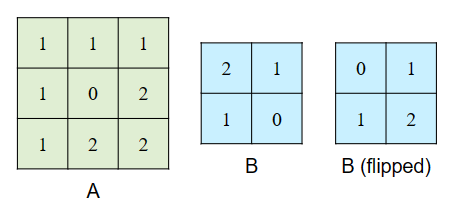
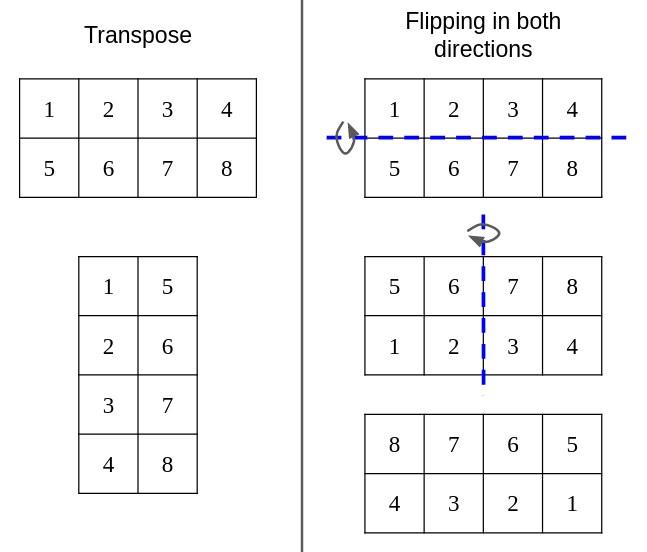
1. You begin by flipping matrix B in both dimensions. Note that flipping matrix B in both dimensions is NOT the same as transposing the matrix. Flipping an MxN matrix results in an MxN matrix. Transpose results in an NxM matrix.

2. Once flipped horizontally and vertically, overlap matrix B in the top left corner of matrix A. Perform an element-wise multiplication of where the matrices overlap and then add all of the results together to get a single value. This is the top left entry in your resultant matrix.
3. Slide matrix B to the right by 1 and repeat this process. This continues until any part of matrix B no longer overlaps with matrix A. When this happens, move matrix B to first column of matrix A and down by 1 row.
4. Repeat the entire process until reaching the bottom right corner of matrix A. You have now convolved matrix A and B. (click the image for a larger version)

You can assume that the height and width of matrix B are less than or equal to the height and width of matrix A.

Note: The output matrix has different dimensions from its input matrices. We'd recommend working out some examples to see how the dimensions of the output matrix is related to the input matrices.

Implementation

Helpful resources: Background: Matrices, Background: Task

Implement convolve in compute_naive.c. You may assume that b_matrix will smaller or equal to a_matrix (that is, if a_matrix is m by n and b_matrix is k by l, then k < m and l < n).

convolve
Arguments	matrix_t* a_matrix	Pointer to the first vector.
	matrix_t* b_matrix	Pointer to the second vector.
	matrix_t** output_matrix	Set *output_matrix to be a pointer to the resulting matrix. You must allocate memory for the resulting matrix in convolve.
Return values	int	0 if successful, -1 if there are any errors.

Testing and Debugging

Helpful resources: Background: Testing Framework, Background: Directory Structure, Background: Testing, Background: Debugging

To run the staff provided tests for this task:

make task_1 TEST=tests/test_tiny
make task_1 TEST=tests/test_small
make task_1 TEST=tests/test_large

If you don't have the tests, please pull the starter first!

If you'd like to create additional tests, please refer to the testing framework section for creating tests as well as the testing and debugging sections for instructions on running tests.

Make sure to create tests of different sizes and dimensions! The autograder will test a wide range of sizes for both correctness and speedup.

Task 2: Optimization

At this point, you should have a complete implementation in compute_naive.c. You will implement all optimizations in compute_optimized.c.

Task 2.1: SIMD

Helpful resources: Lab 7, Discussion 9, Homework 9

Optimize your naive solution using SIMD instructions in compute_optimized.c. Not all functions can be optimized using SIMD instructions. For this project, we're using 32-bit integers, so each 256 bit AVX vector can store 8 integers and perform 8 operations at once.

As a reminder, you can use the Intel Intrinsics Guide as a reference to look up the relevant instructions. You will have to use the __m256i type to hold 8 integers in a YMM register, and then use the _mm256_* intrinsics to operate on them. Make sure you use the unaligned versions of the intrinsic, unless your code aligns the memory to use the aligned versions.

Note: if your implementation of convolve relies on any helper functions, you will want to also convert those to use SIMD instructions as well. Don't forget to implement any tail case(s)!

Hint: You will want to check out the instructions in the AVX family of intrinsic functions, as it may help greatly with certain operations during the convolution process. We understand that there are a lot of functions, but it is a useful skill to be able to read documentation and find information relevant to your task.

Task 2.2: OpenMP

Helpful resources: Lab 7, Discussion 10, Homework 9

Optimize your solution from task 2.1 using OpenMP directives in compute_optimized.c. Not all functions can be optimized using OpenMP directives. You can find more information on OpenMP directives on the OpenMP summary card.

Task 2.3: Algorithmic Optimizations

If your solution from task 2.2 doesn't meet your desired speedups, there is probably room for algorithmic optimizations! This section is a bit more open-ended than the previous two subtasks, since the specific algorithmic optimizations depend on your existing solution and algorithm.

Task 2.4: Testing and Debugging

Helpful resources: Background: Testing Framework, Background: Directory Structure, Background: Testing, Background: Debugging

To run the staff provided tests for this task (note: for this task, you should use make task_2 instead of make task_1):

make task_2 TEST=tests/test_tiny
make task_2 TEST=tests/test_small
make task_2 TEST=tests/test_large

If you don't have the tests, please pull the starter first!

If you'd like to create additional tests, please refer to the testing framework section for creating tests as well as the testing and debugging sections for instructions on running tests. In order to receive full credit, your code should achieve the speedups listed in the benchmarks section of the spec.

Task 3: Open MPI

Helpful resources: Lab 7, Discussion 10, Homework 10

Up until this point, you've been using the provided coordinator_naive.c as the coordinator with a small number of tasks. However, coordinator_naive.c does not have any PLP capabilities and we can optimize it for a workload that includes a larger number of tasks.

1. Implement an Open MPI coordinator in coordinator_mpi.c.

• The structure of the code will be similar to the Open MPI coordinator you wrote in homework 10 and discussion 10.

2. Copy your existing compute functions in compute_optimized.c to compute_optimized_mpi.c, and make any changes necessary to further improve the speedup.

The execute_task function may be helpful here:

execute_task
Arguments	task_t *task	A task_t struct representing the task to execute.
Return values	int	0 if successful, -1 if there are any errors.

Testing and Debugging

Helpful resources: Background: Testing Framework, Background: Directory Structure, Background: Testing, Background: Debugging

To run the staff provided tests for this task (note: for this task, you should use make task_3 instead of make task_1 or make task_2):

make task_3 TEST=tests/test_tiny
make task_3 TEST=tests/test_small
make task_3 TEST=tests/test_large

If you don't have the tests, please pull the starter first!

If you'd like to create additional tests, please refer to the testing framework section for creating tests as well as the testing and debugging sections for instructions on running tests. In order to receive full credit, your code should achieve the speedups listed in the benchmarks section of the spec.

Unfortunately, gdb is not extremely helpful for parallel programs. We recommend using printfs throughout your program to verify that variables contain values you'd expect. We also recommend first testing your optimized compute with the naive coordinator first since it is easier to debug.

Task 4: Partner/Feedback Form

Congratulations on finishing the project! This is a brand new project, so we'd love to hear your feedback on what can be improved for future semesters.

Please fill out this short form, where you can offer your thoughts on the project and (if applicable) your partnership. Any feedback you provide won't affect your grade, so feel free to be honest and constructive.

Benchmarks

There are two types of benchmarks:

• Optimized: uses your compute_optimized.c and the staff coordinator_naive.c
  • These benchmarks are run with a limit of 4 threads for OpenMP.
• Open MPI: uses your compute_optimized_mpi.c and your coordinator_mpi.c
  • These benchmarks are run with a limit of 1 thread for OpenMP and configures Open MPI to use 4 processes.

Speedup Requirements

Speedup Requirements
Name	Folder Name	Type	Speedup
Random	test_ag_random	Optimized	8.10x
		Open MPI	4.70x
Increasing	test_ag_increasing	Optimized	7.78x
		Open MPI	3.30x
Decreasing	test_ag_decreasing	Optimized	8.00x
		Open MPI	3.93x
Big and Small	test_ag_big_and_small	Open MPI	2.68x

Performance Score Calculation

The score for the performance portion of the autograder is calculated using the followed equation: score = log(x) / log(t), where x is the speedup a submission achieves on a specific benchmark, and t is the target speedup for that benchmark.

Submission and Grading

Submit your code to the Project 4 Gradescope assignment. Make sure that you have only modified compute_naive.c, compute_optimized.c, compute_optimized_mpi.c and coordinator_mpi.c.

The score you see on Gradescope will be your final score for this project. By default, we will rate limit submissions to 4 submissions for any given 2 hour period. We may adjust this limit as the deadline approaches and if there is significant load on the autograder, but we will always allow at least one submission per hour.

Appendix: Helper Functions in io.o

We've provided a few helper functions in io.o. However, we've only provided the object file that will be linked with your program at link time. We are not providing the source code for these functions since it may give away solutions for other projects.

read_tasks
Arguments	char *input_file	Path to the input file (the input.txt file).
	int *num_tasks	Set *num_tasks to the number of tasks in the input file.
	task_t ***tasks	Set *tasks as an array of task_t *s, each pointing to a task_t struct representing a task.
Return values	int	0 if successful, -1 if there are any errors.

get_a_matrix_path
Arguments	task_t *task	Pointer to the task.
Return values	char *	Matrix A's path for the given task.

get_b_matrix_path
Arguments	task_t *task	Pointer to the task.
Return values	char *	Matrix B's path for the given task.

get_output_matrix_path
Arguments	task_t *task	Pointer to the task.
Return values	char *	The output matrix's path for the given task.

read_matrix
Arguments	char *path	Path to read the matrix from.
	matrix_t **matrix	Sets *matrix to the matrix stored at path.
Return values	int	0 if successful, -1 if there are any errors.

write_matrix
Arguments	char *path	Path to read the matrix from.
	matrix_t *matrix	The matrix to write to path.
Return values	int	0 if successful, -1 if there are any errors.

Appendix: (Optional) Video Processing

Viewing Output

Since the hive machines are headless (i.e. they don't have a desktop), you need to copy the GIFs locally before you can open them.

1. Find the path to the output GIF. This is generally ~/61c-proj4/tests/name_of_your_test/outX.gif. For example, the output file of the staff provided test_gif_kachow_blur would be located at ~/61c-proj4/tests/test_gif_kachow_blur/out0.gif.

• This assumes that you cloned your repo as 61c-proj4 in the project setup. If this is not the case, replace 61c-proj4 with the name of your folder.
• ls and cd may be helpful here for navigating your files on the hive machines.

2. Open a new terminal on your local machine.

3. In the new terminal window, navigate to the folder you'd like to save the GIF to.

4. Run the following command, where cs61c-??? is your instructional account username, and path_to_gif is the path from step 1.

   scp cs61c-???@hive1:path_to_gif .
   

The file should now be accessible on your local machine, and you can open it with your image viewer of choice.

Appendix: (Optional) Convolutions

The content in this appendix is not in scope for this course.

Convolutions are a mathematical operation that have wide-ranging applications in signal processing and analysis, computer vision, image and audio processing, machine learning, probability, and statistics. Common applications include edge detection in images, adding blur (bokeh) in images, adding reverberation in audio, and creating convolutional neural networks.

This appendix will only give an overview of the 1D discrete time convolution. Discrete time means that a function is only defined at distinct, equally spaced integer indexes. Also, the explanations below are very fast and can be complicated, so it is ok to not understand convolutions for this project. For a much deeper understanding of convolutions and how they interact with signals, be sure to take EE120.

With that, let’s jump in 😈

Mathematically, a convolution is a type of function multiplication that determines how much the two overlap. In real world applications though, a convolution is how a system responds to a signal. A signal can be any mathematical function, and a system can be anything that takes in this function and provides an output. This output is also in the form of a function.

We can describe signals and systems like so:

x(t) -> H -> y(t)

Where x(t) and y(t) are functions, and H is the system.

Important qualities of a system that we’ll need for convolution are linearity and time-invariance.

Linearity: One aspect of linearity is that if you feed a signal into a system that has been multiplied by some constant, it will respond with the original output signal multiplied by the same constant.

αx(t) = x̂(t) -> H -> ŷ(t) = αy(t)

Additionally, linearity means that if you pass in a sum of signals, the system will output a sum of their corresponding outputs.

x_1(t) + x_2(t) = x̂(t) -> H -> ŷ(t) = y_1(t) + y_2(t)

Putting the two together:

αx_1(t) + βx_2(t) = x̂(t) -> H -> ŷ(t) = αy_1(t) + βy_2(t)

Time-Invariance: Time-Invariance means that if you feed a time shifted input into a system, it will respond with an equally time shifted output.

$αx(t - T) = x̂(t) -> H -> ŷ(t) = αy(t - T)$

Going forward, the systems we examine will only be linear and time-invariant (LTI).

In order to determine how a system will respond to any signal, an impulse can be passed into the system. The impulse function used is known as the Kronecker Delta, and it is defined like so:

x(t) = 1 iff t = 0, else x(t) = 0 ∀ t | t ≠ 0

Going forward, this function will be denoted as: 𝛿(t).

An important property of 𝛿(t) is that when it is multiplied by another function x(t), the result is a new function that is 0 everywhere except for t = 0 where it equals x(0). This is due to 𝛿(t) being 0 everywhere except for t = 0 where 𝛿(t) = 1. This can be written as:

x(t)𝛿(t) = x(0)𝛿(t)

This property still holds when 𝛿(t) is shifted by some value T, so more generally:

x(t)𝛿(t - T) = x(T)𝛿(t-T)

This means that we can collect a single value of a function at any integer time value t just by multiplying the function with a shifted 𝛿(t). Knowing this, we can reconstruct x(t) by adding together the functions containing a single point. That means x(t) can be represented as a sum of scaled delta functions like so:

∑x(T)𝛿(t-T) from T = -∞ to ∞ = … + x(-1)𝛿(t + 1) + x(0)𝛿(t) + x(1)𝛿(t - 1) + …

This is a very useful property of the delta function because instead of passing x(t) itself into a system, we can pass in this sum and gain more insight about the output, but first we must investigate how a system responds to 𝛿(t).

When 𝛿(x) is fed into the system, the output is known as the impulse response.

𝛿(t) -> H -> h(t)

There are a few methods for finding h(t), one of which being physically testing the system with an impulse and measuring the output. Knowing this, let’s see what happens when we pass in the scaled sum of delta functions. We know that because the system is LTI, passing in a sum of scaled inputs will result in a sum of corresponding scaled outputs. Additionally, inputs shifted in time will give the corresponding output time shifted by the same value. This means that:

x(t) =  … + x(-1)𝛿(t + 1) + x(0)𝛿(t) + x(1)𝛿(t - 1) + … -> H ->  … + x(-1)h(t + 1) + x(0)h(t) + x(1)h(t - 1) + … = y(t)

The output can then be expressed as ∑x(T)h(t-T) from T = -∞ to ∞, and this is defined as the convolution of x(t) and h(t) and the operator is denoted with the symbol *. The system responded to x(t) by convolving it with the impulse response. Convolution is also a commutative operation, although the proof of this is left as an exercise for the reader. The sum also shows why one of the vectors in exercise 1.2 must be flipped to directly multiply the vectors together. x(T) begins evaluating at -∞ and is multiplied with h(t-T) which begins at +∞, so without flipping, you must have two pointers, one starting at the beginning of the first vector and the other at the end of the second vector, progressing in the opposite direction. By flipping h(t - T) and getting h(-t + T), it is also evaluated from -∞ to +∞, allowing for the two vectors to be directly multiplied to find the output at t. Since convolution is commutative, it doesn’t matter which vector is flipped.

As a final point, notice that the input sum of ∑x(T)𝛿(t-T) from T = -∞ to ∞ is also convolution, one between x(t) and 𝛿(t), and it equals x(t). That means that 𝛿(t) is the identity for convolution, and x(t)*𝛿(t) = x(t) for any x(t).